Part 1 – Basics of Pulse Code Modulation (PCM)
To me, when explaining the Ring DAC – or DACs in general – it makes sense to start with the basics of digital audio from the perspective of PCM (all subjective debates on quality aside, I think anyone versed on the topic can agree it is the most prevalent format). For those already in the know, don’t worry, I’ll be getting on to the fun stuff soon!
Sound is analogue, and it’s created when varying amounts of pressure cause air particles to vibrate and bump into one another – a process that produces longitudinal waves. This is much like what would happen if you asked two people to stretch out a slinky between them and had one person push the slinky forward. Their push would cause a ‘ripple’ to pass through the slinky, pushing each coil forward and compressing it into the next. Each time a new coil is pushed forward, the previous one would retract back – or ‘rarefy’ – and this wave of compression would move through the slinky until it reached the other end.
This same process happens with sound. When a person speaks, their vocal cords excite and push the air surrounding them back and forth, and this creates longitudinal waves in the air. When these longitudinal waves reach an endpoint – the human ear – the changes in air pressure are translated into electrical signals that the brain perceives as sound.
The whole purpose of recorded music is to take these variations in air pressure and store them in such a way that they can later be reproduced by a transducer such as headphones or loudspeakers, to enable a listener to hear the original audio event as it happened.
In today’s world, the most common way this takes place is to capture a musical performance with one or more microphones (which convert the kinetic energy in the particles of the air to electrical energy, a voltage) and use an Analogue to Digital Converter (ADC) to convert this into a format that can be stored by computers, streamed over the internet and so forth.
An ADC looks at the voltage that is coming in from the studio equipment like a microphone or mixing desk and determines how high the voltage is, storing it as a group of binary digits (1s and 0s), called a ‘word’. There are two key variables in PCM digital audio: The sample rate (how frequently samples are taken) and the bit depth (how many bits – 1s and 0s – are in each audio sample word).
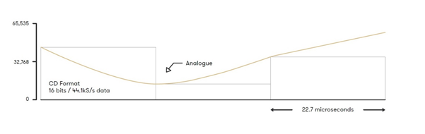
This diagram shows how an analogue sound wave can be represented with 16-bit 44,100 samples per second PCM encoding.
Bit Depth
A lot of digital audio, including CDs, use a bit depth of 16 bits. This bit depth means that the ADC can have one of 65535 possible values at any given point. Bit depth refers to how many bits can be used to describe the absolute position of a sound wave in digital audio recording. It is generally accepted that the human ear can perceive equivalent to 20-bits of dynamic range, which equates to around 140dB (the upper limit being the threshold of pain). CD audio, in its 16-bit format, will achieve around 96dB of dynamic range (the difference between the loudest and quietest volumes that can be sampled). Through the use of dither, the addition of low-level noise to the signal, this dynamic range can be increased beyond 120dB, a significant improvement. Moving to a hi-res format like 24-bit, this dynamic range increases to 144dB – assuming the equipment is actually capable of working in true 24-bit.
It is a common misconception that 24-bit audio simply records louder and quieter sounds than is possible with 16-bit audio, but this is not the case. Instead, the same range of loudest to quietest is measured, but with 24-bit sampling it is done with considerably more steps than with 16-bit. This means the absolute value of the waveform at any given point can be much better represented.
Imagine for a moment trying to measure the height of a particular window on a skyscraper. In one case, you can only measure in increments of 1 metre. If the window is 10.7m high, you could round down to 10m or up to 11m, but in either case there would be a degree of error.
Now imagine the same situation, but this time you are able to use increments of 0.2m. The window is again 10.7m high. You are still unable to measure the exact height of the window, but being able to round to 10.6m or 10.8m brings you much closer to the actual value.
This is in essence what happens when increasing the bit depth of digital audio. You are able to measure the absolute value of the waveform with much greater precision, which has the effect of reducing what is known as quantisation noise in the audio. Quantisation noise is the audible noise which is generated by the error in the measurement. Essentially what this means is that when you measure the 10.7m high window as 11m, that 0.3m error in the measurement creates negative audible effects in audio.
When working with hi-res audio, each additional bit which is added to the bit-depth of a signal halves the quantisation error, quarters the error power, and thus reduces quantisation noise by 6dB.
Sample Rates
If the human ear can only hear up to 20,000Hz, is there any reason to use sample rates higher than 20,000Hz? As it happens, yes. One of the most important aspects of digital audio is the Nyquist Theorem, which specifies that the digital audio samples need to be taken at a minimum of twice the highest frequency one is trying to record in the original analogue audio. As the upper limit of human hearing is widely accepted as 20,000Hz, digital audio needs to be sampled at at least 40,000Hz to be able to reproduce the full range of human hearing. For reasons that will be discussed later (related to the digital filtering inside a Digital to Analogue Converter), full range recordings are sampled slightly higher than this, with CD audio being sampled at 44,100Hz. The rate at which these samples is taken is referred to as the sample rate, defining how many samples are used per second.
Further to this, running digital audio at higher rates allows for gentler anti-aliasing filters to be used (don’t worry, this will all be covered in future posts – these filters are incredibly important and warrant their own full explanation). In essence, higher sample rates and gentler filtering mean that the filters will be affecting the audio less, with fewer effects like pre- and post-ringing impacting the sound quality.
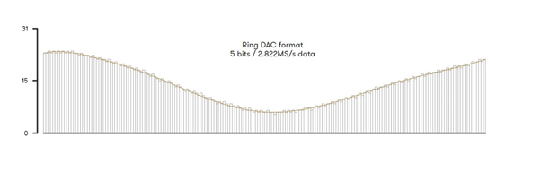
These two numbers, the sample rate and the bit depth, are what define PCM audio. The display of a dCS product playing back PCM data will show 24/192 when playing back a PCM stream with 192kHz 24-bit data.
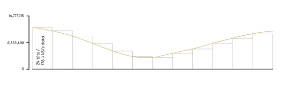
This diagram shows how an analogue sound wave can be represented with 24-bit 176,400 samples per second PCM encoding. The sample rate being higher than CD audio above allows for a greater representation across the X axis of this graph, whereas the higher bit-depth allows for the exact amplitude of the wave to be more accurately represented with each sample – the Y axis.
Now we’ve covered the basics of PCM, we’ll move on to another widely used format, Pulse Density Modulation (the basis of DSD), before moving on to digital to analogue conversion.
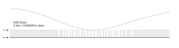
Part 2 - Basics of Pulse Density Modulation (DSD)